This example can be developed on the blackboard for 30 to 50 minutes, depending on how thorough the explanations given to the students are.
Example: Fourier series of a symmetrical square pulse train
Problem Statement
Develop the Fourier series of the signal $f(t)$.
Approach
Signal characteristics
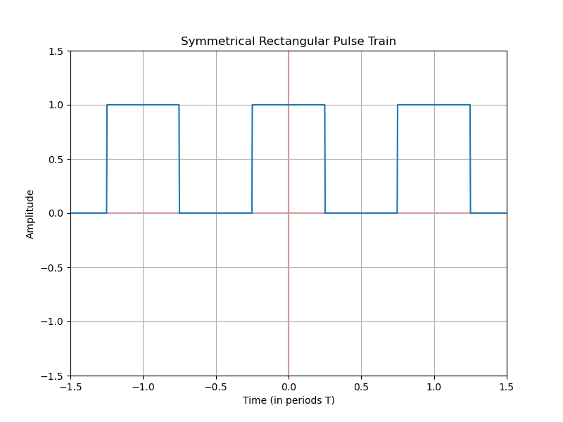
We have a periodic time function, which could be generated by a square wave oscillator. It’s periodic with a symmetrical duty cycle, meaning it stays high for as long as it stays low.
Period
The repeating signal has a period from $-T/2$ to $T/2$. We could choose a different period as a period is just a segment of the repeating signal. We could also choose from $0$ to $T$. However, due to the characteristics of the Fourier transform, choosing a symmetrical period will simplify the integration.
Sum of pulses
The function can be written as a sum of pulses. This expression is also called a generating function.
- Pulse Width: The pulse width is $T/2$.
- Generating Function: It’s the function that generates the repeating signal: $\pi\left( \frac{t}{T/2} \right)$
- Displacement: The first pulse is centered at the origin, and the following pulses are displaced by a quantity $T$.
- Analytic Expression: $f(t)=\sum_{n=-\infty}^\infty \pi\left( \frac{t-nT}{T/2}\right)$
Solution
Coefficients $d_n$
To get a Fourier series, we need to calculate the coefficients $d_n$ first: $d_n=\frac{1}{T} \int_{-\infty}^{\infty} f(t) e^{-j 2\pi n f_0 t} \, dt$
Periodic Function
We integrate the generating function over a period. We choose a period $T$ centered at the origin: $d_n=\frac{1}{T} \int_{-T/2}^{T/2} \pi\left( \frac{t}{T/2} \right) e^{-j 2\pi n f_0 t} \, dt$
Simplifying the Integration Limits
The periodic function is either 1 or 0; we integrate within the limits where it equals 1: $d_n=\frac{1}{T} \int_{-T/4}^{T/4} e^{-j 2\pi n f_0 t} \, dt$
Integration
The integration is straightforward; $j$ is considered as a constant: \begin{align} d_n &= \frac{1}{T}\cdot \frac{-1}{j 2\pi n f_0} \left[ e^{-j 2 \pi n f_0 t} \right]_{-T/4}^{T/4}
&= \frac{1}{T}\cdot \frac{-1}{j 2\pi n f_0} \left[ e^{\frac{-j 2 \pi n f_0 T}{4}} - e^{\frac{+j 2 \pi n f_0 T}{4}}\right] \end{align}
Simplifying
Knowing that the fundamental frequency $f_0$ is the inverse of the period $f_0=T^{-1}$: \begin{equation} d_n = \frac{-1}{j 2\pi n } \left[ e^{\frac{-j \pi n }{2}} - e^{\frac{+j \pi n }{2}}\right] \end{equation}
Complex Expression of the Sine
If we recall the expression of the sine as a subtraction of complex exponentials (equ:trig_sin_exp) and the properties of an odd function: \begin{equation} d_n = (-1/πn) \cdot sin(-πn/2) = sin(πn/2)/(πn) \end{equation}
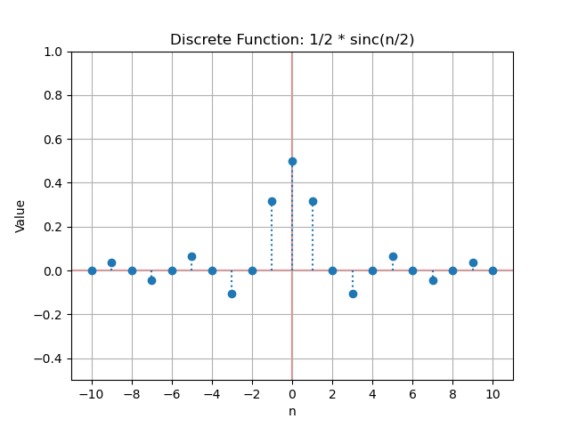
Cardinal sine
Another way to write the previous function is as a normalized cardinal sine function, defined by its application in signal theory. \begin{equation} sin(πn/2)/(πn) = \frac{1}{2} \cdot sin(πn/2)/(πn/2) = \frac{1}{2} sinc(πn/2) = \frac{1}{2}\cdot sinc_n(n/2) \end{equation}
Coefficient values
To give values to the coefficients d_n, we replace the value of n by a series of natural integers. In this case, the only problem is the value 0, which is undefined; however, by taking the limit, it is easy to see that it is 1 (by applying L’Hôpital’s rule, or considering the identical slopes of the functions sin(n) and n at the origin).
| $n$ | $sinc_n(n/2) = (2/πn) \cdot sin(πn/2)$ | $d_n=1/2 \cdot sinc_n(n/2)$ |
|---|---|---|
| 0 | 1 | 1/2 |
| 1 | 2/π | 1/π |
| 2 | 0 | 0 |
| 3 | -2/(3π) | -1/(3π) |
| 4 | 0 | 0 |
| 5 | 2/(5π) | 1/(5π) |
| 6 | 0 | 0 |
| 7 | -2/(7π) | -1/(7π) |
Values of the negative coefficients
The sinc function is an even function; for negative values of $n$ it takes the same values as for positive values of $n$.
Fourier series
Now that we have the coefficients $d_n$, we can write the terms of the Fourier series by applying the expression. \begin{equation} f(t) = \left[… -1/(3π) \cdot e^{-j2π3f0t} + 1/π \cdot e^{-j2πf0t} + 1/2 + 1/π \cdot e^{j2πf0t} -1/(3π) \cdot e^{j2π3f0t} + …\right] \end{equation}
Real function of the Fourier series
Although the previous expression is already a Fourier series, it is a sum of complex exponentials; we can rearrange the expression to get the same function expressed in sines and cosines.
Group terms
We can group symmetrical terms: \begin{equation} f(t) = [1/2 + 1/π \cdot (e^(j2πf0t)+e^(-j2πf0t)) - 2/(3π) \cdot (e^(j2π3f0t)+e^(-j2π3f0t)) + …] \end{equation}
Series formed by cosines
Now it’s easier to see that the series is formed by cosines. Applying the expression of the cosine as the sum of complex exponentials: \begin{equation} f(t) = [1/2 + 2/π \cdot (e^(j2πf0t)+e^(-j2πf0t))/2 - 2/(3π) \cdot (e^(j6πf0t)+e^(-j2π3f0t))/2 + …] = [1/2 + 2/π \cdot cos(2πf0t) - 2/(3π) * cos(6πf0t) + …] \end{equation}
Summation
\begin{equation} f(t) = 1/2 \cdot \sum_{n=1}^\infty ((-2(-1)^n) / (2n-1)\pi) \cdot cos(2 \cdot (2n-1) \cdot \pi f0 t) \end{equation}
Graphical representation**
If we superimpose the original signal on the terms of the obtained series, we see that the series resembles the original signal more and more as we add terms.
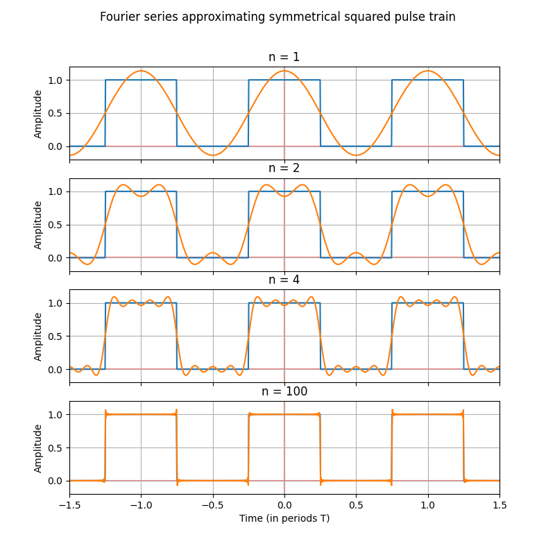
As we add terms to the series, it increasingly resembles the original signal.
Conclussions
The Fourier series has allowed us to express a periodic signal, which was a piecewise function (a square wave), as the sum of sine and cosine functions, i.e., harmonic functions, which are easier to handle mathematically.
This analysis is used in many areas of engineering, such as linear system analysis, signal and system analysis, digital signal processing, telecommunications, electronics, acoustics, and so on.
The Fourier coefficients are a representation in the frequency domain of the original signal, which is also of interest in many contexts. In this example, we have observed that the odd frequencies have more importance, while the even frequencies do not contribute.
Finally, it is important to highlight that the Fourier series converges to the original signal when the number of terms tends to infinity. However, in practice, a fairly good approximation of the original signal can be obtained with a finite number of terms, as demonstrated in the last figure. The choice of the number of terms to use depends on the level of precision required and the computational limitations.